1. Introduction

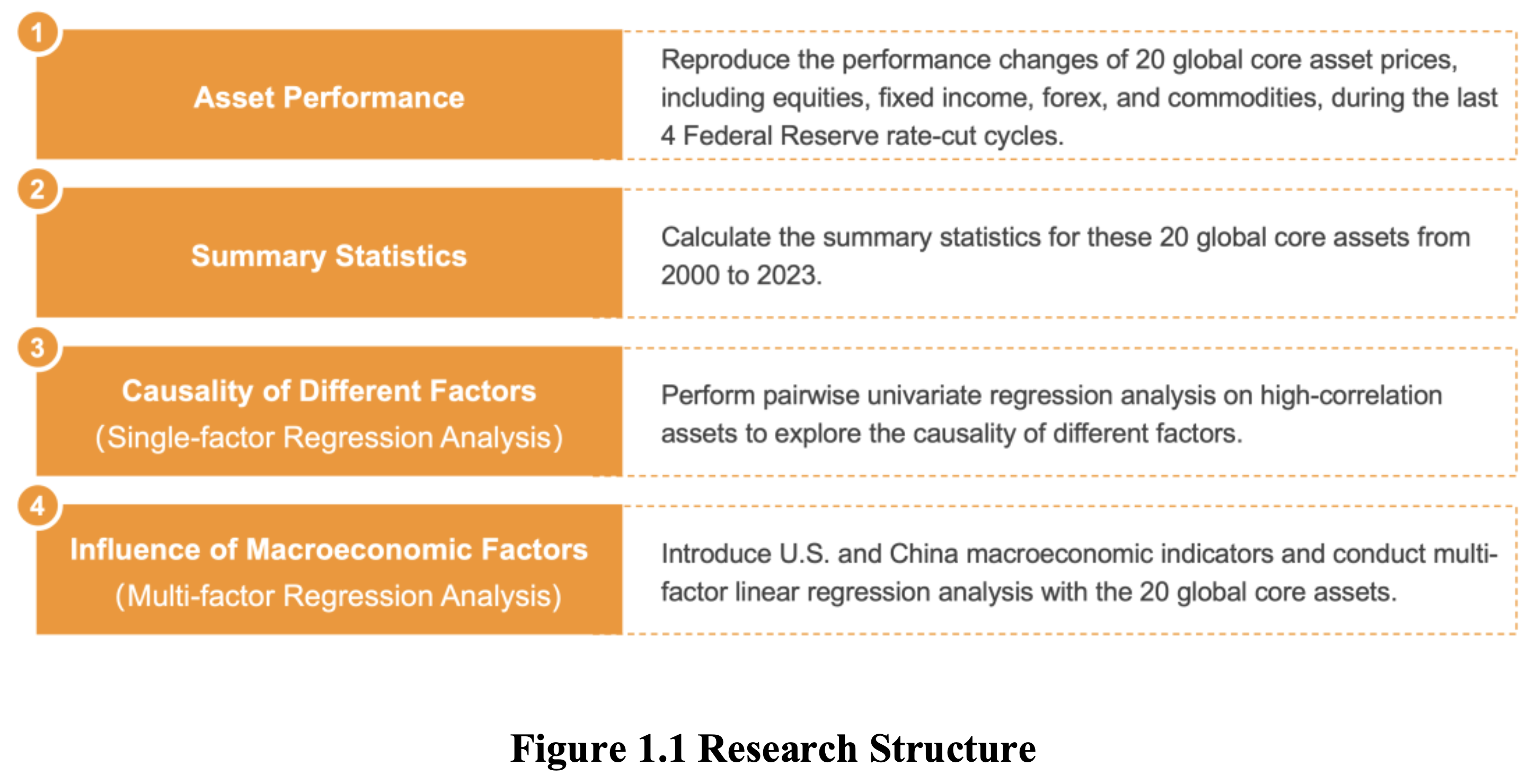
This report presents a quantitative analysis of the performance of 20 global core assets, including equities, fixed income, forex, and commodities. Firstly, the performance changes of these assets during the last 4 Federal Reserve rate-cut cycles are reproduced and compared with Haitong Securities research report. Secondly, the summary statistics for these assets are calculated to identify long-term trends and anomalies in asset behavior. Thirdly, pairwise univariate regression analysis is conducted on high- correlation assets to explore the causality of different factors. Finally, U.S. and China macroeconomic indicators are added to conduct multi-factor linear regression analysis with these 20 global core assets. Through this comprehensive approach, the report aims to enrich understanding of the interplay among global assets and macroeconomic factors.

2. Methodologies

The tasks in this report are completed by a comprehensive Python-based code architecture designed for financial quantitative analysis (Figure 2.1). This architecture focuses on achieving full-process automation and modularization, ensuring each component functions independently while maintaining seamless connectivity through standardized interfaces. The architecture comprises five principal layers: Data Integration, Data Processing, Modeling, Task, and Application.

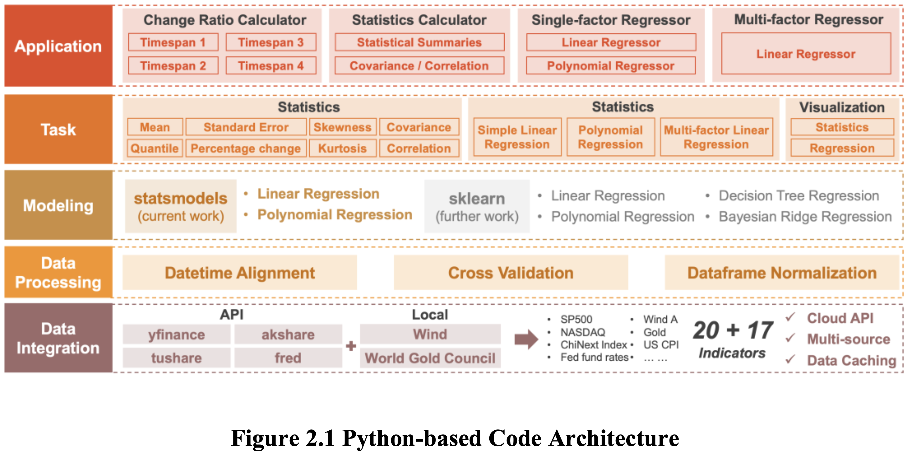
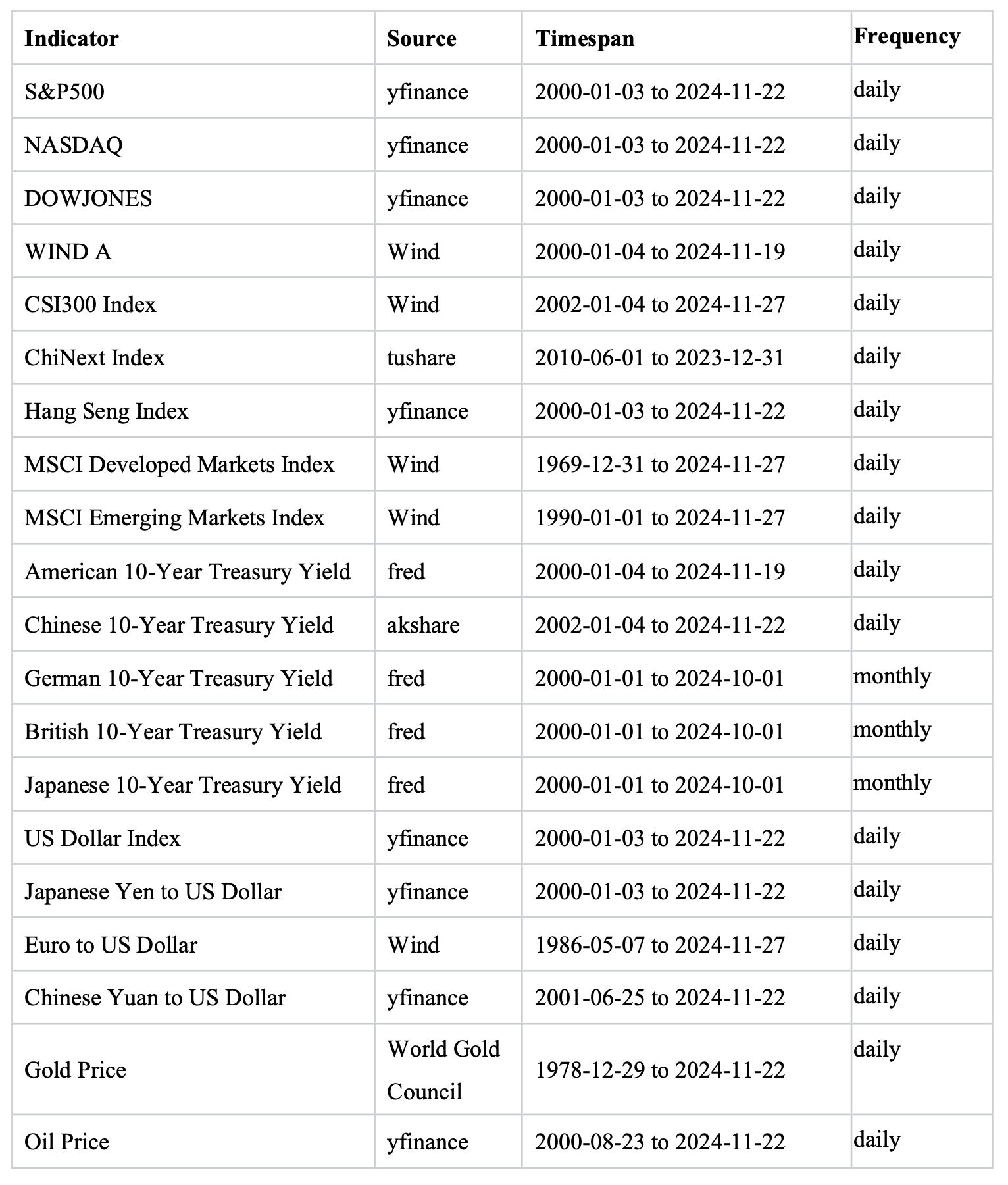
The Data Integration Layer is responsible for aggregating data from diverse sources, including open-source APIs such as yfinance and fred, as well as local databases such as Wind, capturing a wide spectrum of financial and economic indicators. This layer incorporates a caching mechanism procedure to optimize data retrieval efficiency. Comprehensive details regarding data sources, time periods, and frequencies are provided in Appendix A.

Following data aggregation, the Data Processing Layer preprocesses data by executing datetime alignment to ensure synchronized timeframes. Cross-validation techniques are applied to assess the generalizability of models, while normalization processes are employed to standardize datasets, thus preparing them for analysis in subsequent stages.

In the Modeling Layer, advanced analytical models are implemented using libraries such as ‘statsmodels’ and ‘sklearn’. This includes linear regression (both simple and multi-factor), polynomial regression to capture nonlinear dynamics, and complex modeling approaches like decision tree and Bayesian Ridge regression for more intricate analytical tasks.

Despite the comprehensive capabilities of the modeling layer, this report specifically utilizes the ‘statsmodels’ library for linear and polynomial regression because the emphasis of this study is on deriving statistical insights rather than price prediction. Future work could expand the scope by using ‘sklearn’ for data regression, which is more conducive to machine learning applications. Such an approach would involve establishing distinct training and test sets to enhance prediction accuracy and model validation.

Within the Task Layer, three primary categories of analysis are defined: statistical metrics calculation, regression analysis, and analysis visualization. Each task is implemented as a function and can be easily called by other layers.

The Application Layer provides tools for answering specific financial research questions. It includes functions like asset change ratio calculator, single-factor and multi-factor regressors. In summary, this architecture has modular design for easy expansion, supports multiple tools and data sources, and is designed for automation and efficiency.

3. Findings and Discussion

3.1 Asset Performance During a Fed Rate Cut Cycle

3.1.1 Reproduction and Comparison

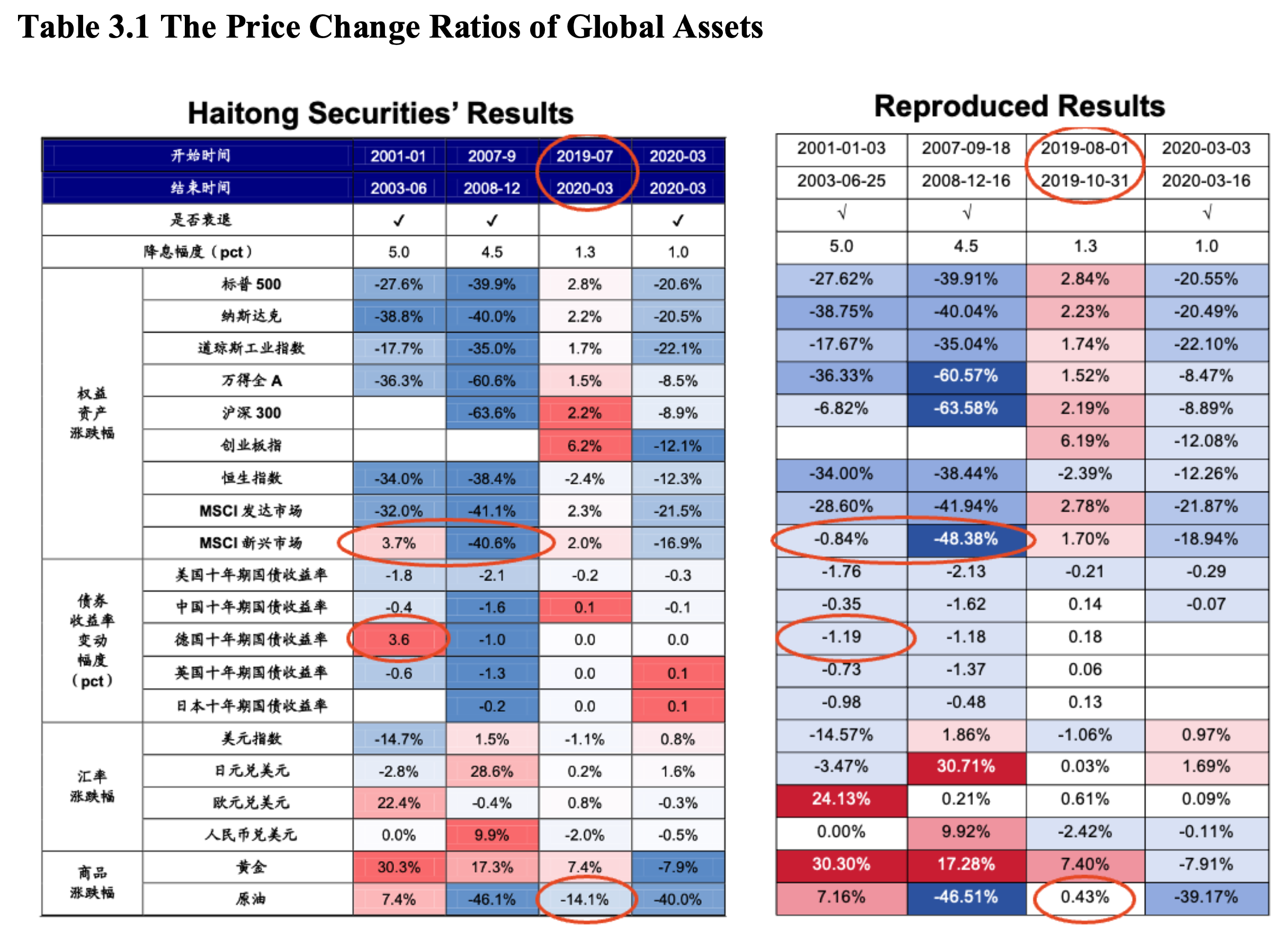
Based on Haitong Securities’ report*, we recalculated the price change ratios of the 20 global assets during the four most recent Federal Reserve rate-cutting cycles. Our findings were cross validated against the report’s data as shown in Table 3.1. Combined the report’s context, we identified an error in the third rate-cutting cycle timeframe, which should be corrected to “2019-08-01 to 2019-10-31” (as shown in Table 2 in the original report), rather than “2019-07 to 2020-03”. In addition, our analysis revealed several differences in asset price data:

• The first two change ratios for MSCI Emerging Markets Index have some difference, potentially attributable to differences in data sources or quality.
• Significant disparities in the first change ratio for German 10-year Treasury Yields and the third change ratio for Oil, with opposing trends. We vitrificated the data, which suggests potential calculation errors in the Haitong Securities report.
• Due to the availability of only monthly frequency data for German, UK, and Japanese 10-year Treasury Yields, change ratios could not be calculated for the fourth interval, which spans only 13 days.
• We supplemented missing data from the Haitong Securities report for the CSI 300 and Japanese 10-year Treasury Yields in the first time interval. Additionally, as the ChiNext Index was established in 2009, data for the first two time intervals are unavailable. This comprehensive review enhances the accuracy and completeness of the original analysis, providing a more robust foundation for understanding asset price behavior during Federal Reserve rate-cutting cycles.

* Haitong Securities. (2024, August 17). The impact of historical Federal Reserve interest rate cuts on asset prices. Retrieved from https://www.htsec.com/jfimg/colimg/upload/20240819/1724033432062020929.pdf

3.1.2 Analysis of Asset Performance

Equity assets

We can see that the performance of equity assets during the Fed rate cut cycle is not entirely consistent. In the two interest rate reduction cycles of 2001-2003 and 2007-2008, the world’s major stock markets have fallen sharply, the S&P 500, Nasdaq, Dow Jones Industrial Index and other declines are about 20%-40%, and these two interest rate reduction cycles are accompanied by economic recession. In the early period of 2019-2020, the economy was relatively stable, and the stock market performance was also relatively stable. Next, we can compare the impact degree of different markets. From this table, we can see that the US stock market fluctuates greatly in each interest rate cut cycle. Emerging market stock markets, such as MSCI Emerging Market Index, suffered a large decline from 2001 to 2003, and the S&P 500 index fell by 27.62%. The Nasdaq fell 38.75 percent, and the Dow Jones Industrial Average fell 17.67 percent. During this period, the United States experienced the bursting of the Internet bubble, the economy fell into recession, corporate earnings fell sharply, investor confidence fell, and the stock market underwent a sharp correction. The 2007-2008 rate cuts took place against the backdrop of the global financial crisis, when the bursting of the bubble in the US housing market triggered a large number of financial institution failures, an outbreak of systemic risks, and a heavy hit to the stock market. The Chinese stock market also suffered A huge decline in 2007-2008 due to the impact of the global financial crisis. The Wende All-A Index fell 60.57% and the CSI 300 index fell 63.58%.

Bonds

The US 10-year Treasury bond yield has declined to varying degrees in each rate cut cycle, which is in line with the expectation that the Fed’s rate cut will lead to an overall decline in market interest rates. Yields on 10-year government bonds in other major economies also mostly fell or fluctuated downward, though to a lesser extent than in the United States. In the interest rate cut cycle, the overall performance of the bond market is relatively stable, as a safe-haven asset, when the economic recession or uncertainty increases, investors’ demand for bonds increases, pushing bond prices up and yields down.

Exchange Rate

Dollar trend: The US dollar index fell sharply during the 2001-2003 rate cut cycle, while it was relatively stable or slightly higher during the 2007-2008 and March 2020 rate cut cycles. This is related to the global economic situation and the relative strength of other economies. Let’s look at the exchange rate changes of other currencies against the US dollar. Among them, the euro appreciated sharply against the US dollar from 2001 to 2003, the Japanese yen appreciated sharply against the US dollar from 2007 to 2008, and the RMB also appreciated significantly against the US dollar from 2007 to 2008.

Product

In each rate cut cycle, the gold price generally performed better, except for the decline in March 2020, which was affected by the liquidity crisis caused by the epidemic, and the other periods had varying degrees of increase. As a safe-haven asset, gold tends to be more popular with investors in times of economic instability and loose monetary policy. However, the performance of crude oil prices in different interest rate reduction cycles varies greatly, with relatively stable or slightly rising prices in 2001-2003 and 2019-2020, and sharp declines in 2007-2008 due to the impact of the global financial crisis.

3.2 Summary Statistics

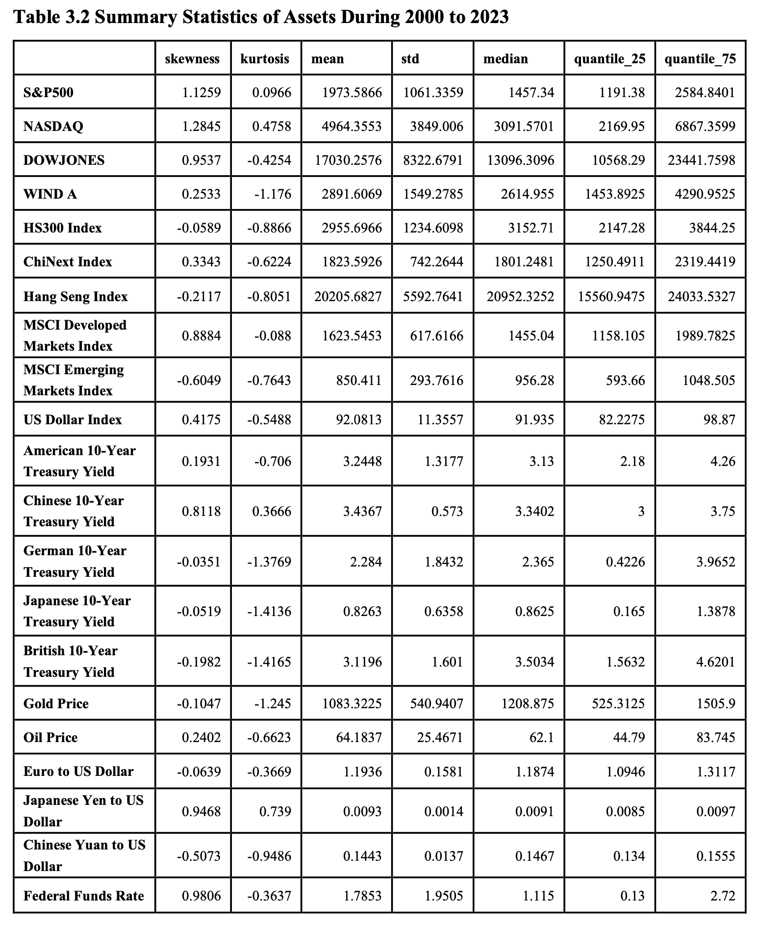
We calculated the statistical indicators of 20 assets from 2000 to 2023. From the Table 3.2, we can see that there are significant differences in skewness, kurtosis, mean, and standard deviation among different financial indicators, reflecting their different distribution characteristics and fluctuation degrees. Generally, stock indexes have large fluctuations, and their skewness and kurtosis vary, reflecting the complexity and diversity of the stock market. The fluctuations of treasury bond yields are relatively small, the fluctuations of currency exchange rates are also small, and the fluctuations of gold prices among commodity prices are large.

3.2.1 Correlation

The correlations between pairs of indicators are calculated, including both covariance and correlation. The focus is primarily on correlation, as it is standardized to range between -1 and 1. The correlation values are categorized into several groups based on their magnitudes and are represented using five distinct shades of color. The highest correlation values are indicated by orange and dark blue, respectively (Table 3.3).

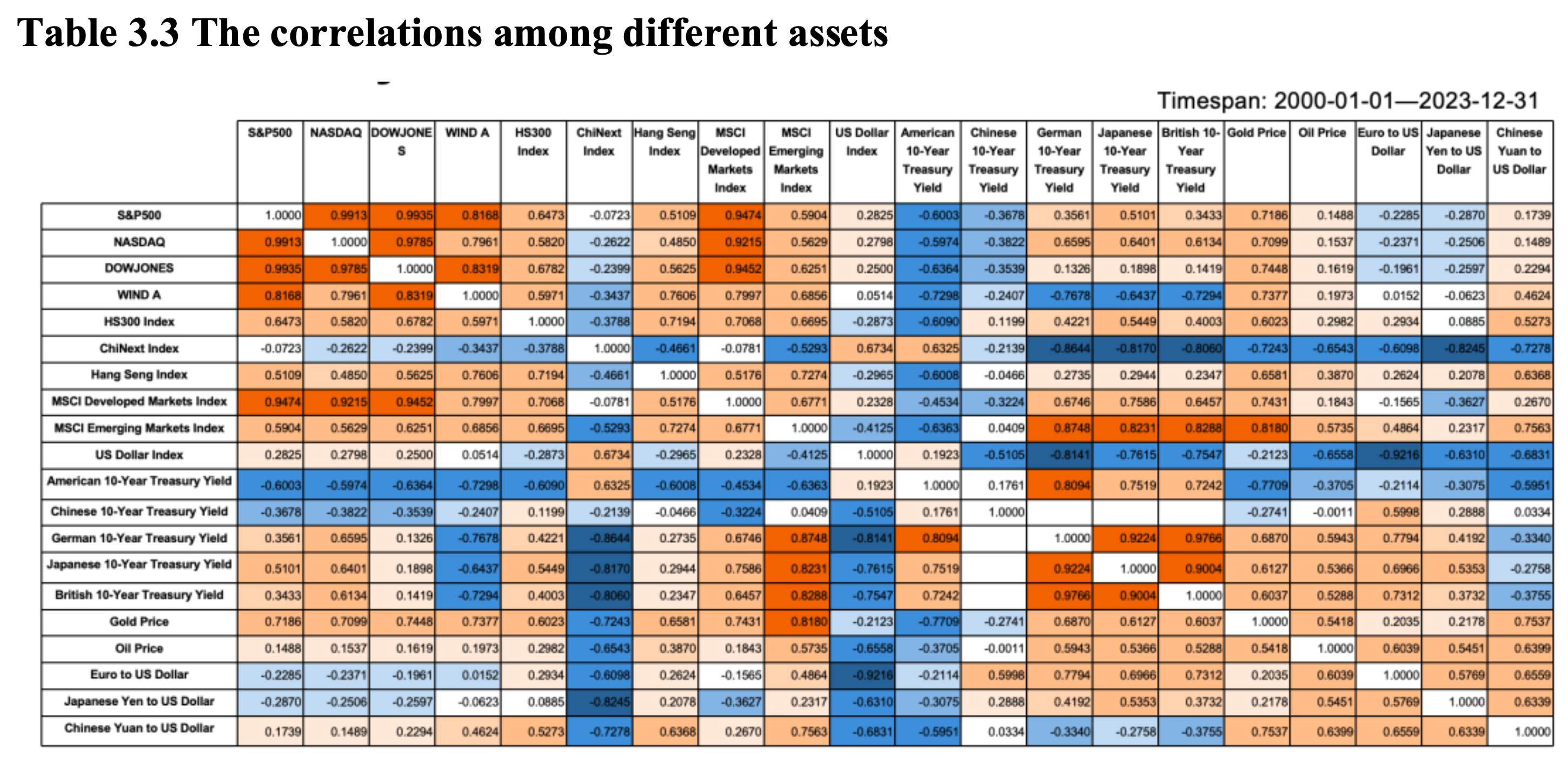
The correlations between indices are analyzed as follows:

• Major US Stock Indices: S&P500, NASDAQ and DOWJONES have a high degree of positive correlation, and the correlation coefficient is above 0.97, indicating that the three major US stock indexes are highly consistent and the overall trend of the market is strong.
• China Stock Indices: The correlation between HS300 Index and WIND A is high, reaching 0.7606, while the correlation between ChiNext Index and other indexes is weak, and even negatively correlated with some indexes, such as S&P500, NASDAQ, DOWJONES, etc. It reflects that the trend of the GEM index is quite different from that of the main board market and the US market, and it is relatively independent.
• Global Stock Indices: The MSCI Developed Markets Index has a high correlation with major U.S. stock indexes and some global stock indexes, indicating a strong correlation with developed markets around the world. The MSCI Emerging Markets Index also has a certain correlation with most stock indexes, and a high correlation with the MSCI Developed Markets Index, indicating that there is a certain interaction between emerging markets and developed markets.
• Stock Indices and Interest Rate: Us stock market and US Treasury yields: There is a significant negative correlation between major US stock indexes and American 10-Year Treasury Yield. For example, the correlation coefficient between S&P500 and American 10-Year Treasury Yield is -0.6003. It indicates that when the yield of US Treasury bonds rises, funds will flow from the stock market to the bond market, which will form a certain pressure on the stock market.
• China Stock Market and China Bond Yields: The correlation between China’s 10-Year Treasury Yield and China’s stock Index is relatively weak, such as the correlation coefficient with HS300 Index is 0.1199, and the correlation coefficient with ChiNext Index is -0.2139. It shows that the fund flow relationship between the Chinese stock market and the national debt market is not as obvious as that in the American market.
• Global Interest Rate: German 10-Year Treasury Yield, Japanese 10-Year Treasury Yield and British 10-Year Treasury Yield are highly positively correlated, and also strongly correlated with some stock indexes. It reflects that there is a certain linkage in the interest rate markets of the world’s major economies.
• Stock Indices and Commodities and Foreign Exchange: Stock indices and Gold: Most stock indexes show a positive correlation with Gold Price. For example, the correlation coefficient between S&P500 and Gold Price is 0.7186, indicating that when market uncertainty increases or economic downside risks are large, the attributes of stocks and gold as safe havens will be highlighted at the same time, and funds will flow to these two markets at the same time.
• Stock Indices and Oil: The correlation between Oil Price and various stock indexes is relatively weak, indicating that the correlation between oil market and stock market is not strong, and the direct impact of oil price fluctuations on the stock market is limited.
• Forex Market and Other Assets: The correlation between the US Dollar Index and most stock indexes and other assets is complicated, and it is mostly negatively correlated with the stock index, and also has a certain negative correlation with the yield of Treasury bonds, while it is negatively correlated with the price of gold, the price of oil, and the exchange rate of euro, yen and RMB against the US dollar. It reflects the special status of the US dollar as the world’s major reserve currency and its complex relationship with various assets.
• Exchange rates: There is a certain positive correlation between the exchange rates of EUR/USD, JPY/USD and RMB/USD, indicating that there is a certain correlation between the exchange rates of major currencies in the world.

3.3 Causality of Different Factors

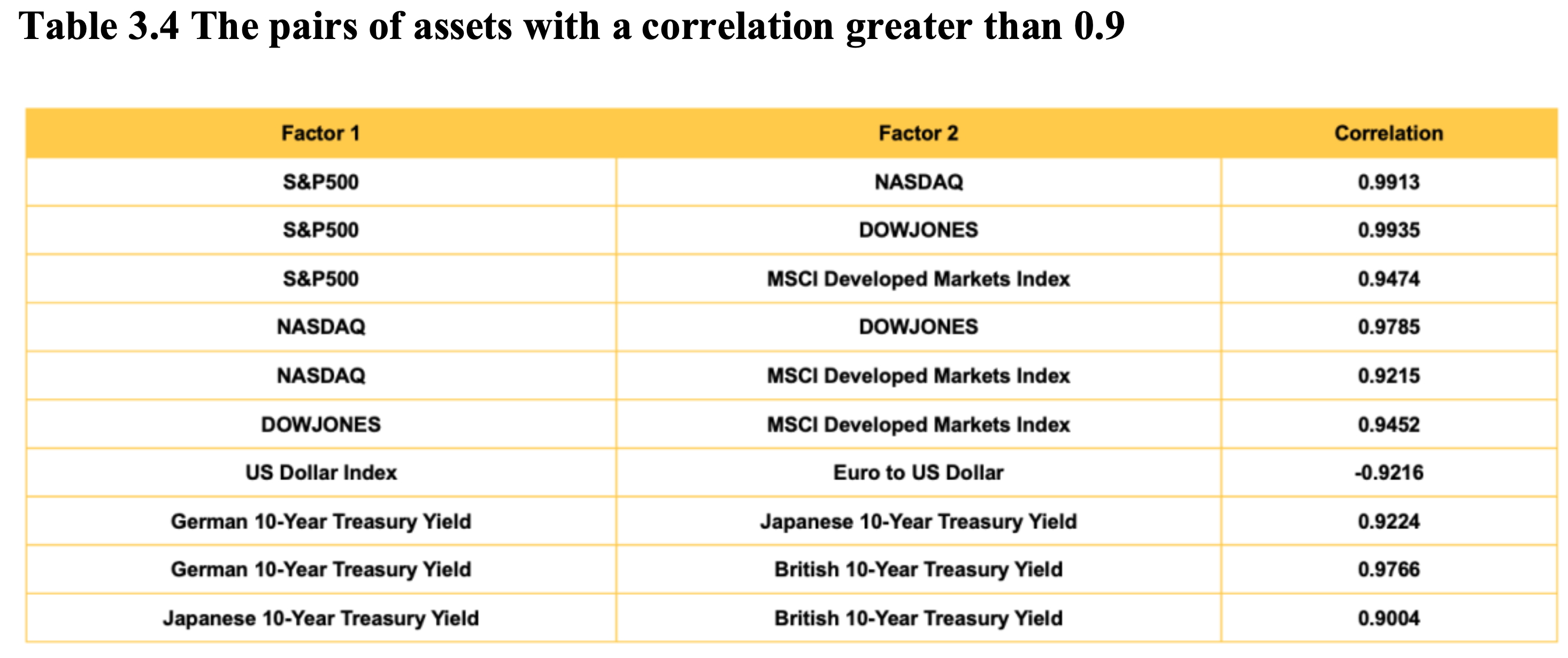
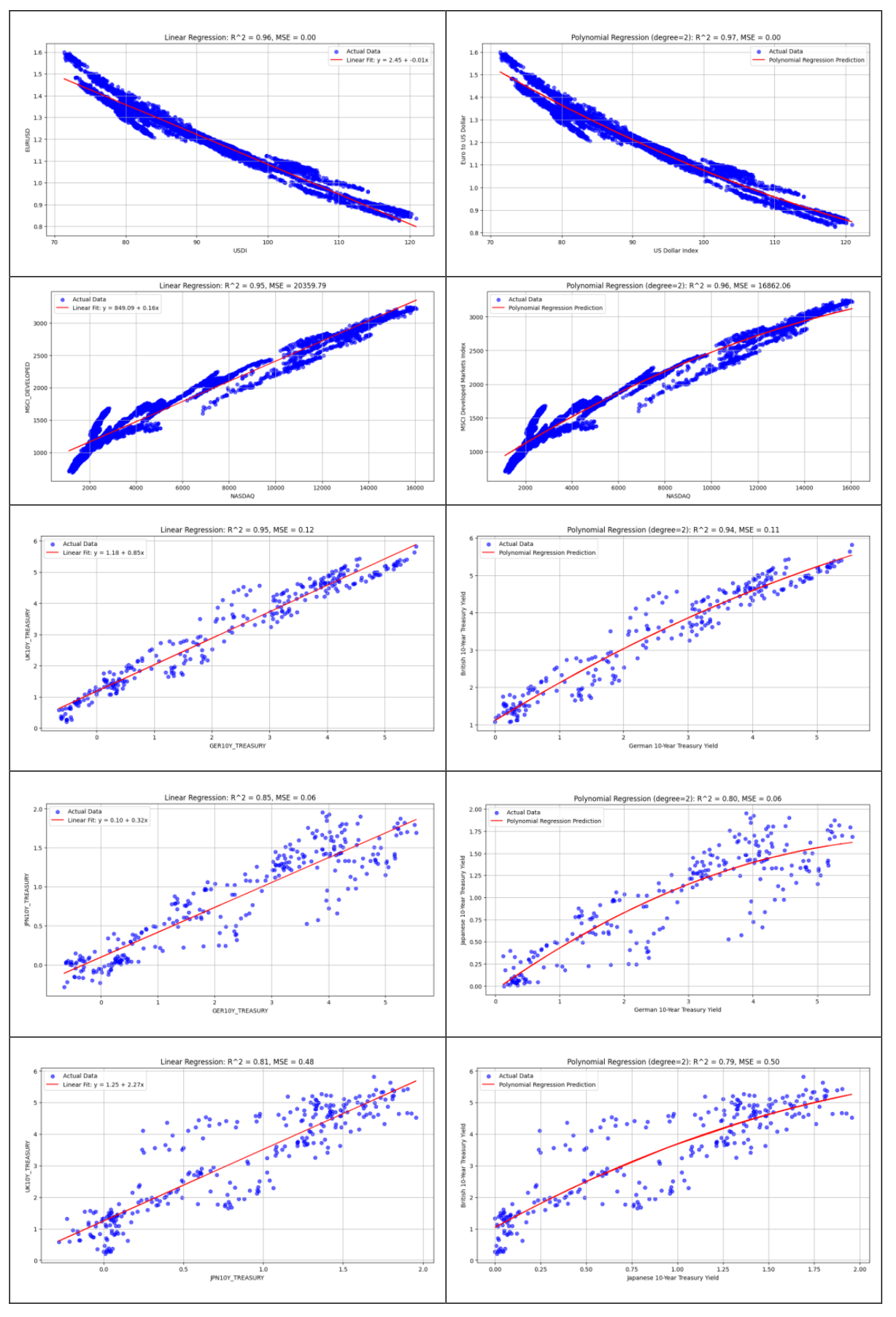
This section adopts regression methods to investigate the causality among different assets. The analysis focuses on pairs of assets with a correlation greater than 0.9, as calculated in the previous section, ultimately identifying 10 pairs for further study (Table 3.4). Notably, strong correlations are observed among the S&P 500, Dow Jones, MSCI Developed Markets Index, and Nasdaq. Similarly, the 10-year Treasury yields of the UK, Japan, and Germany exhibit strong correlations. Additionally, a significant negative correlation is detected between the US Dollar Index and the Euro to US Dollar exchange rate.

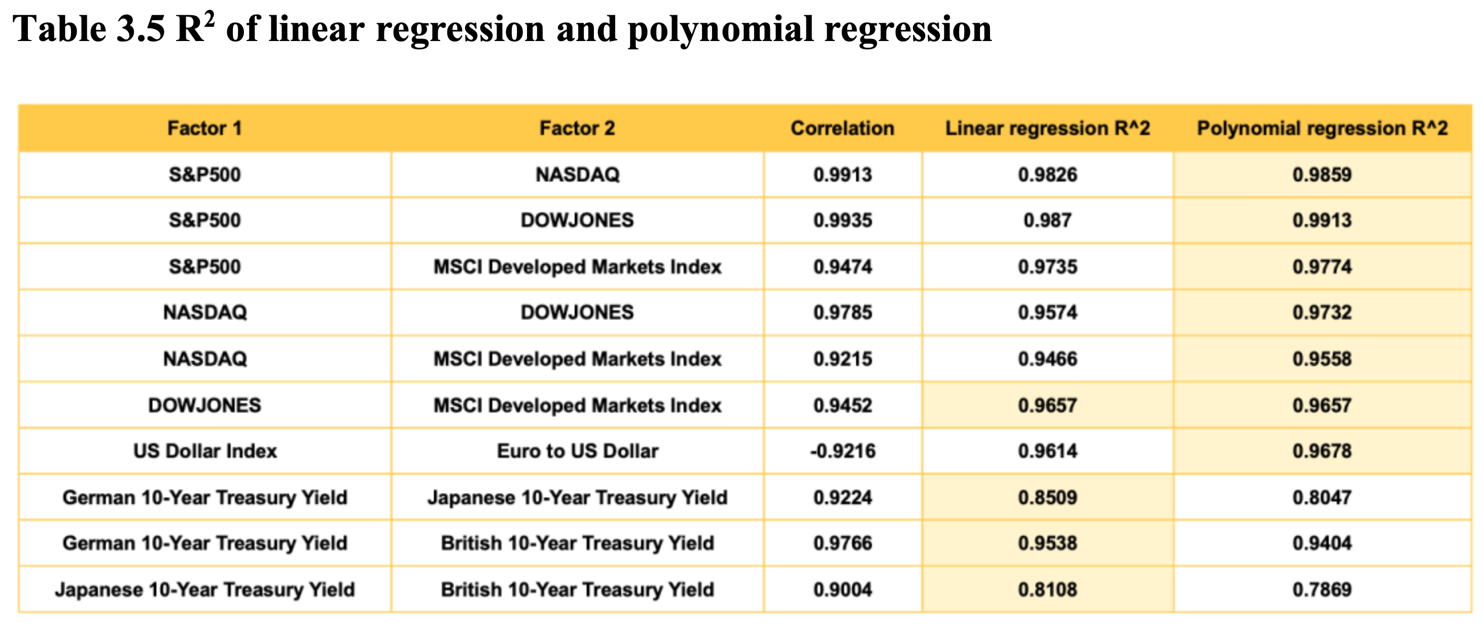
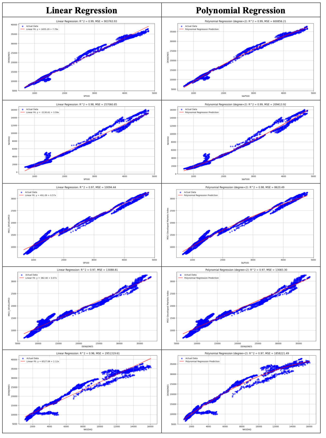
The selected indicators are subsequently examined through both linear and polynomial regression techniques. In implementing polynomial regression, a degree of freedom of 2 is chosen to mitigate the risk of overfitting. It is evident from the analysis that polynomial regression generally offers superior performance, except in the last three data groups, owing to its ability to capture more intricate patterns by trading off degrees of freedom. The discrepancy arises because the last three groups involve 10-Year Treasury Yields with limited monthly data; thus, linear regression suits their simpler patterns, whereas polynomial regression falters due to insufficient data complexity.

Subsequently, representative pairs from the identified 10 pairs are selected to be analyzed deeply, with remaining results presented in the Appendix C.

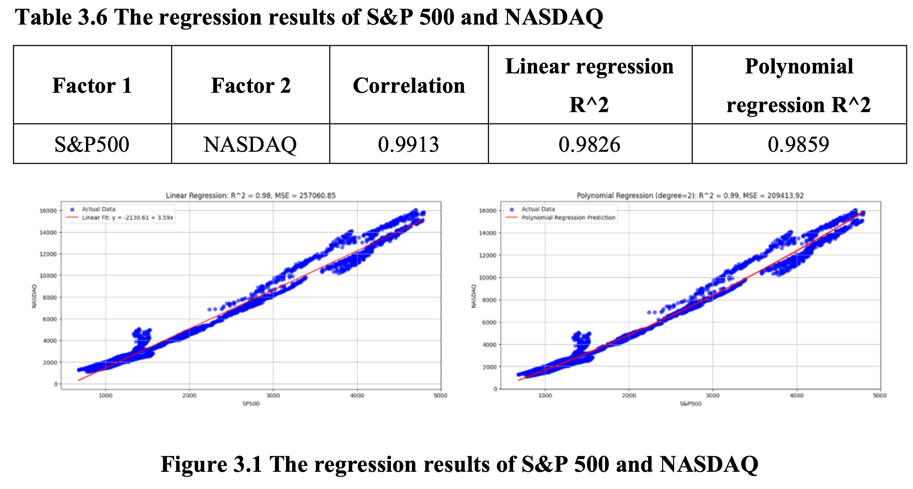
3.3.1 S&P 500 and NASDAQ

This pair exhibits a high positive correlation of 0.9913, with high fitting degree outcomes (Table 3.6, Figure 3.1). It could be explained as the following reasons:

• Market Composition and Focus: Both indices encompass major U.S. corporations, leading to synchronized movements.
• Sector Overlap: Technology and communication services dominate both indices. Investor sentiment shifts, such as strong tech earnings, similarly affect both.
• Market Sentiment and Economic Trends: Both indices react to macroeconomic factors like interest rate changes and economic reports. Growth stocks in both indices benefit from positive economic news but lag during uncertainty or monetary tightening.
• Investor Behavior: Institutional investors frequently adjust allocations between these indices. Gains in one, often led by tech, can drive investment in the other.
• Correlation Over Time: A historically high correlation exists, particularly during tech bull markets, though sector-specific divergences can cause temporary decreases, such as healthcare or finance outpace tech.

3.3.2 DOWJONES & MSCI Developed Markets Index

This pair also exhibits a high positive correlation of 0.9452 (Table 3.7, Figure 3.2). It could be explained as the following reasons:

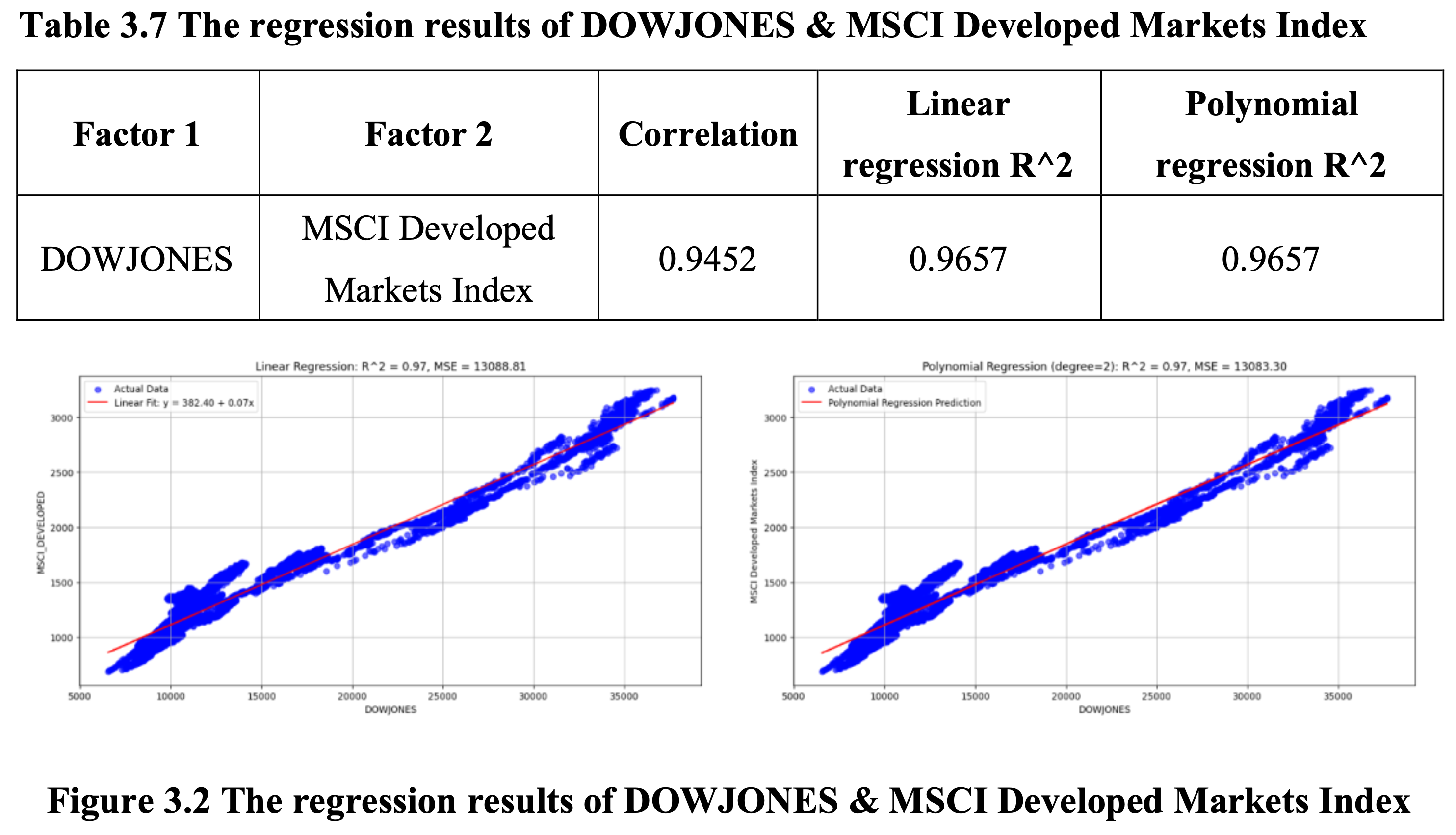
• Industry Leader Effect: DOWJONES and MSCI Developed Markets Index feature industry leaders in their constituent stocks, reflecting global financial prominence. DOWJONES includes top U.S. companies like Microsoft and JPMorgan Chase, representing technological and financial leadership. Similarly, MSCI comprises global leaders, such as Siemens in Germany and Toyota in Japan. These industry leaders, through their adaptive strategies and market influence, drive significant index performance, enhancing their correlation.
• Global Investment Strategy: Institutional investors, informed by macroeconomic and industry analyses, pursue global investment strategies, leading to coordinated capital movements and valuation fluctuations in both indices. This behavior, observed during trends like the global expansion of the new energy sector, strengthens the linkage between DOWJONES and MSCI.
• Global Market Integration: The advanced integration of global markets, propelled by technological, trade, and capital flow liberalization, heightens the interconnectedness of economies. The U.S. economic fluctuations significantly impact export industries of other developed countries. Additionally, global financial market integration, influenced by multinational corporate activities and international monetary policies (e.g., U.S. Federal Reserve actions), increases the consistency in market trends between DOWJONES and MSCI, contributing to their high correlation.

3.3.3 US Dollar Index and Euro to US Dollar

This pair exhibits a high negative correlation of 0.9913, with high fitting degree outcomes (Table 3.8, Figure 3.3). It could be explained as the following reasons:

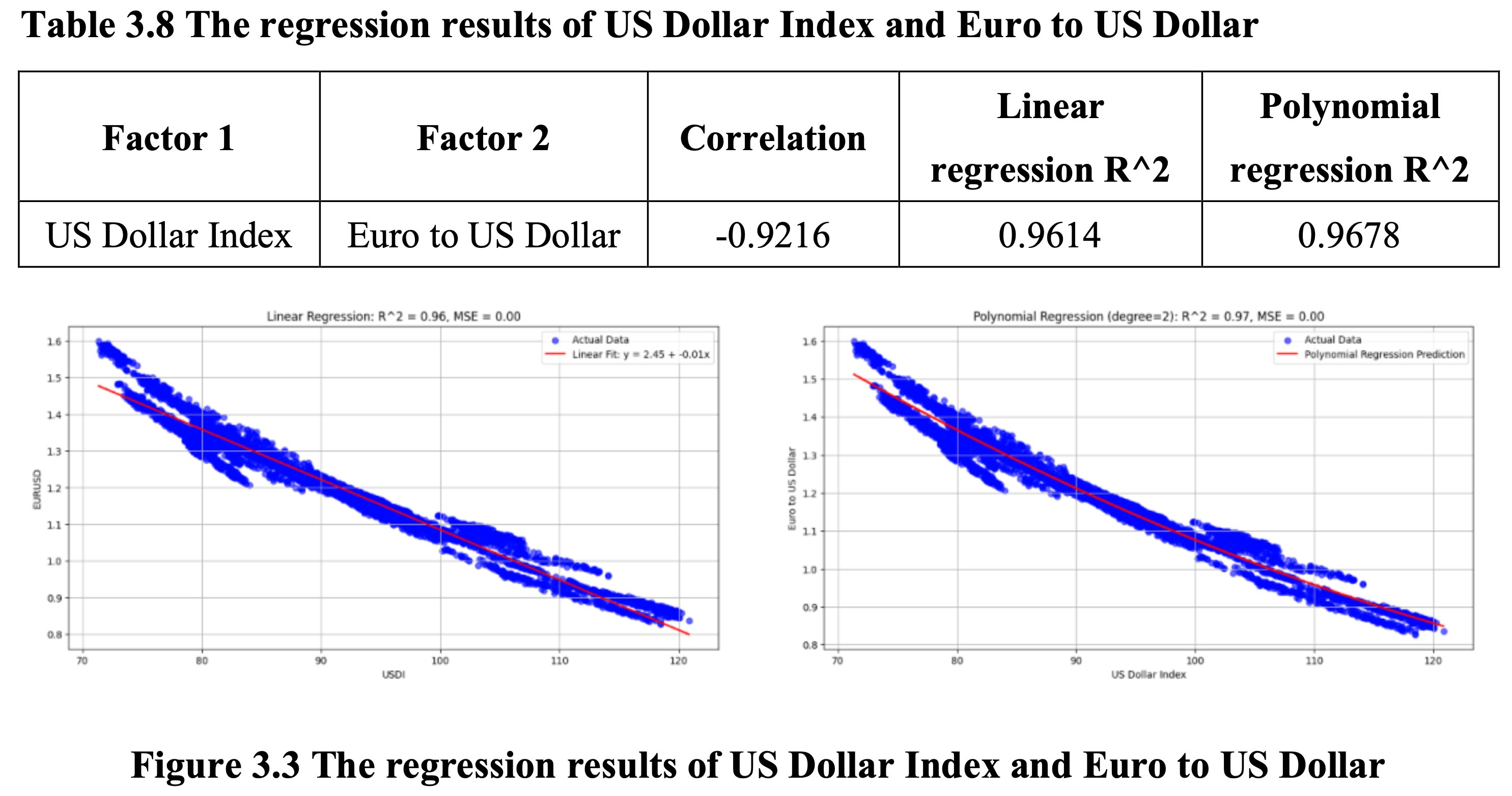
The US Dollar Index is a vital measure of the US dollar’s strength against a basket of major currencies, with the euro comprising a substantial 57.6% of this basket. This significant weighting grants the euro considerable influence over the fluctuations of the Dollar Index. As a key international reserve and payment currency, the euro’s exchange rate is shaped by eurozone economic fundamentals, monetary policy directions, and external market conditions. When the eurozone exhibits robust economic growth, such as increased GDP, stable employment, and controlled inflation, the euro strengthens against the dollar, leading to a decline in the Dollar Index. Conversely, during economic downturns, such as debt crises or recession risks, the euro may depreciate, causing the Dollar Index to rise as the dollar’s relative value increases.

This inherent relationship, driven by the euro’s high weighting in the Dollar Index, underscores the strong negative correlation between the US Dollar Index and the Euro to US Dollar exchange rate. It necessitates that investors closely monitor eurozone economic conditions and policy shifts, considering the direct impact of euro-dollar exchange rate fluctuations on the Dollar Index when evaluating US dollar trends and making forex investment decisions.

3.3.4 Japanese 10-Year Treasury Yield and British 10-Year Treasury Yield

Despite a strong correlation of 0.9004, the linear and polynomial regression fits for this pair are relatively modest (Table 3.9, Figure 3.4), likely due to several factors:

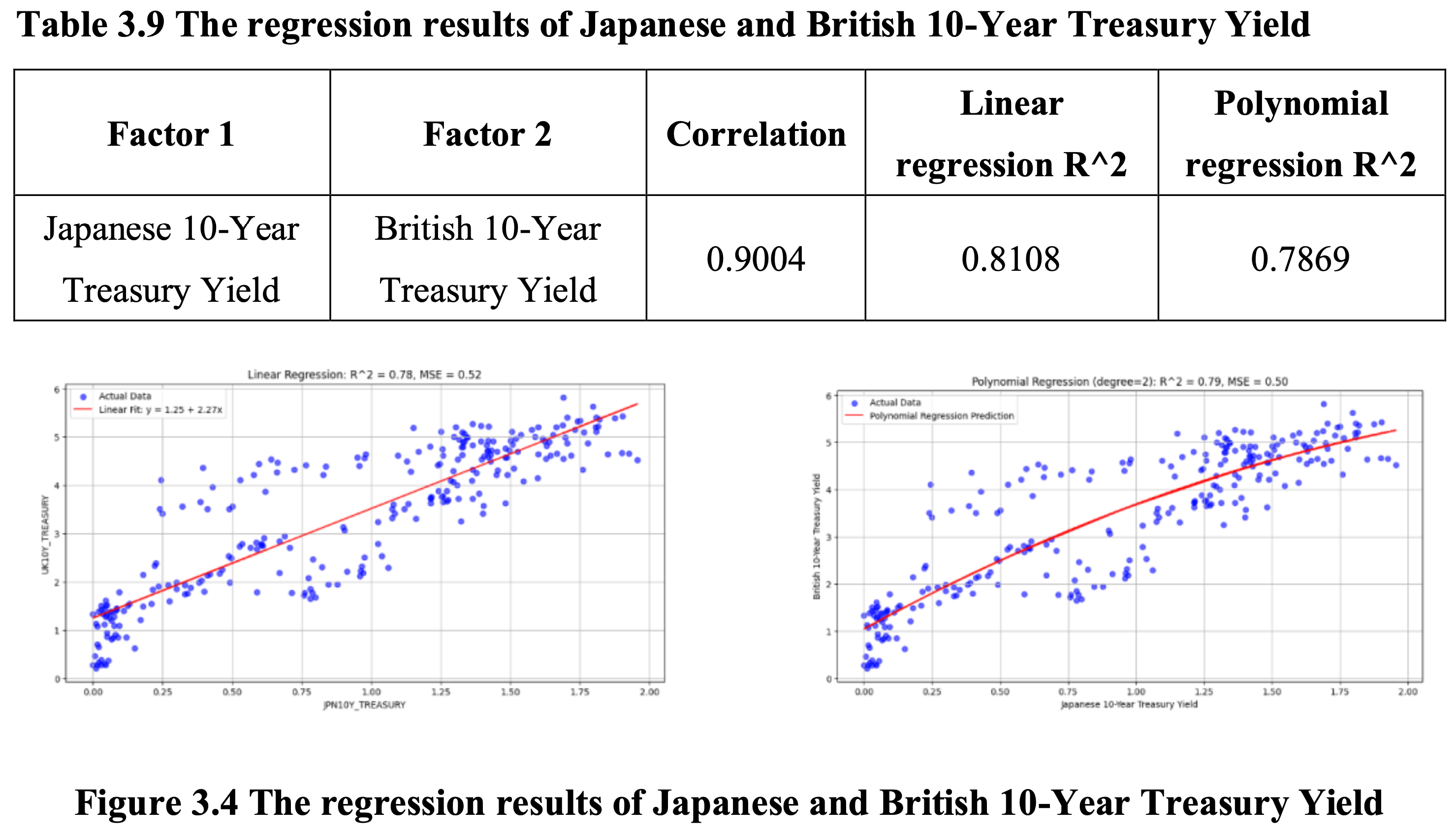
• Influence of External Factors: Government bond yields are affected by complex external factors like monetary policy, economic growth expectations, and inflation. Japan’s prolonged low or negative interest rates and quantitative easing result in consistently low 10-year bond yields. Conversely, the UK adjusts rates based on economic conditions, impacting its 10-year bond yields. Japan’s conservative growth outlook further suppresses its yields, while the UK’s potentially higher growth expectations elevate theirs. Diverging inflation expectations also play a role, causing deviations in yield trends despite high correlation, thereby influencing regression fit.
• Nonlinear Relationship: Though correlational analysis indicates a linear relationship, nonlinear dynamics also exist due to financial market complexities. Events like financial crises or geopolitical tensions can drastically alter investors’ risk preferences, causing nonlinear fluctuations in demand for government bonds. Additionally, factors such as bond issuance, market liquidity, and trading behaviors introduce nonlinear interactions, potentially misaligning linear models with actual yield relationships. This necessitates exploring nonlinear models for accurate depiction.
• Data Fluctuations and Noise: Financial market data, including the Japanese and British bond yields, are prone to fluctuations and noise, influenced by macroeconomic releases, political events, and investor sentiment. Such disturbances create short-term volatility, affecting model fit despite long-term correlation. Trading systems, time differences, and data processing errors exacerbate noise, challenging accurate relationship capture in models. Addressing data fluctuations with preprocessing techniques and robust statistical methods enhances analysis accuracy.

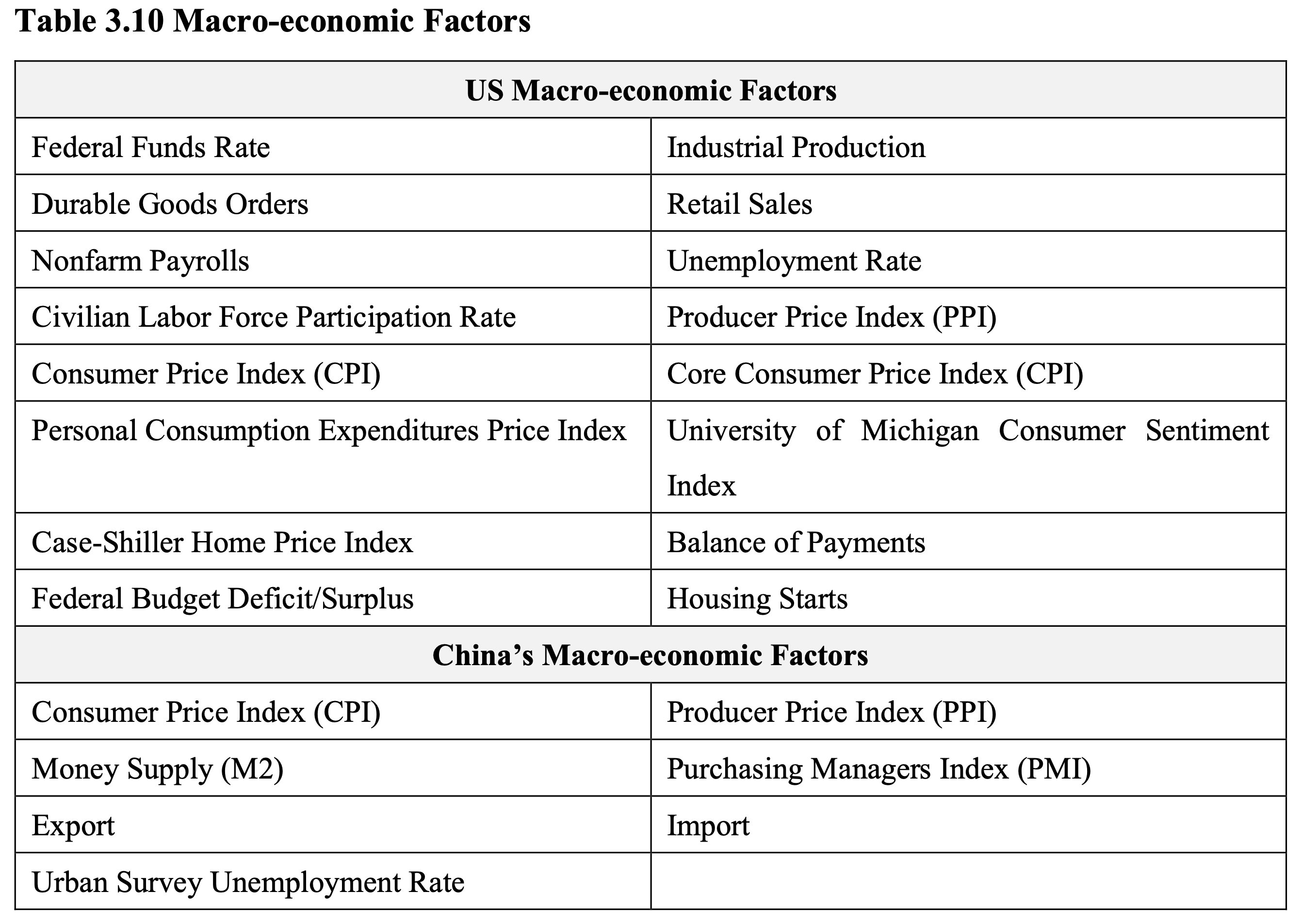
3.4 Influence of Macro-economic Factors

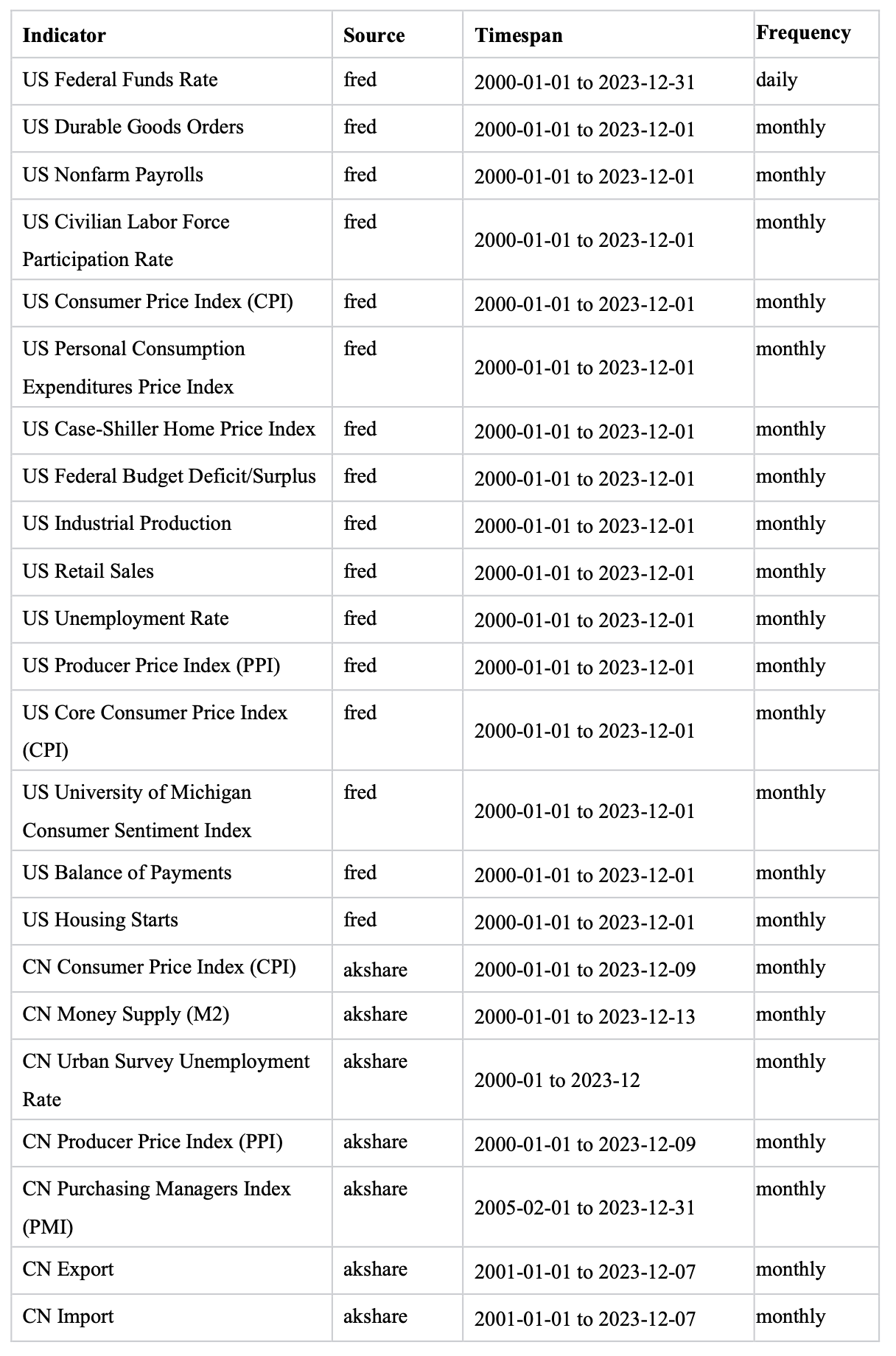
This section explores the impact of macroeconomic indicators on asset prices. Given the global role of the US dollar, the size of the US economy, and the depth of its financial markets, US macroeconomic data is considered to play a critical role in shaping asset prices worldwide. To examine this, 16 US macroeconomic factors were introduced and analyzed through multiple linear regression. For assets from China, due to the independence of China’s monetary policy and differing macroeconomic conditions, a separate multiple linear regression is conducted using 7 China’s macroeconomic indicators. The factors are presented in Table 3.10.

3.4.1 Multi-factors Regression based on US Macroeconomic Indicators

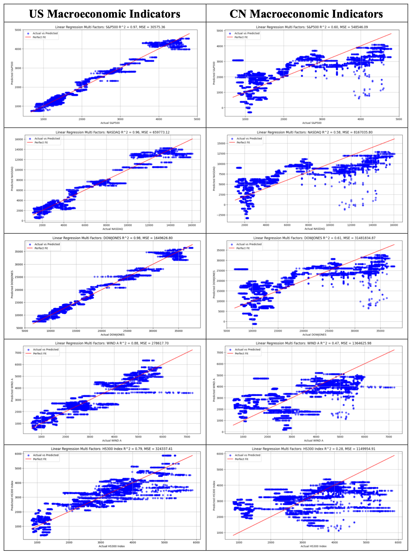
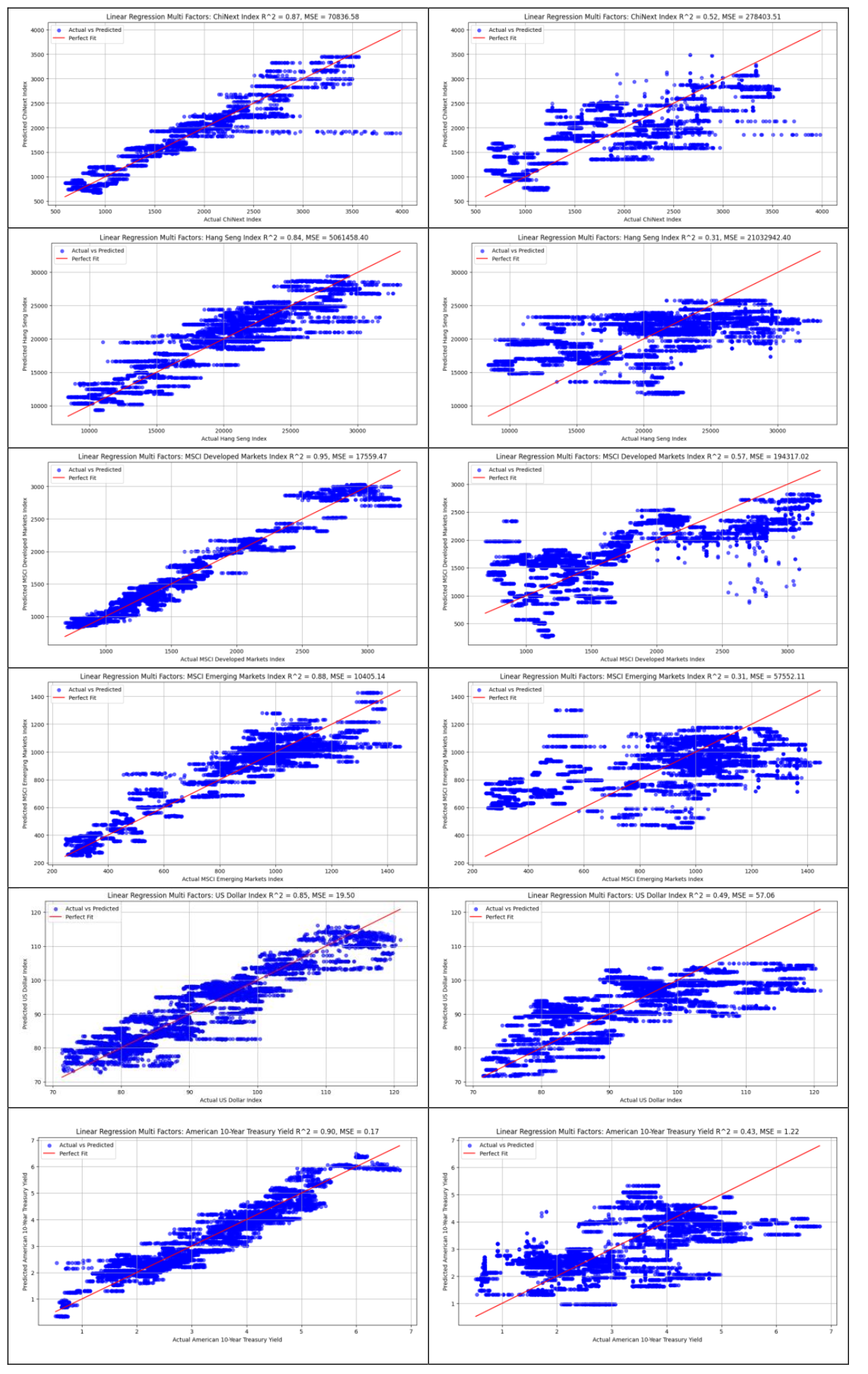
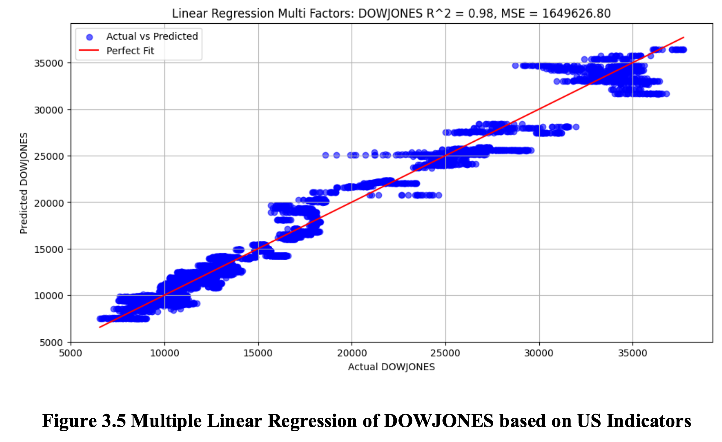
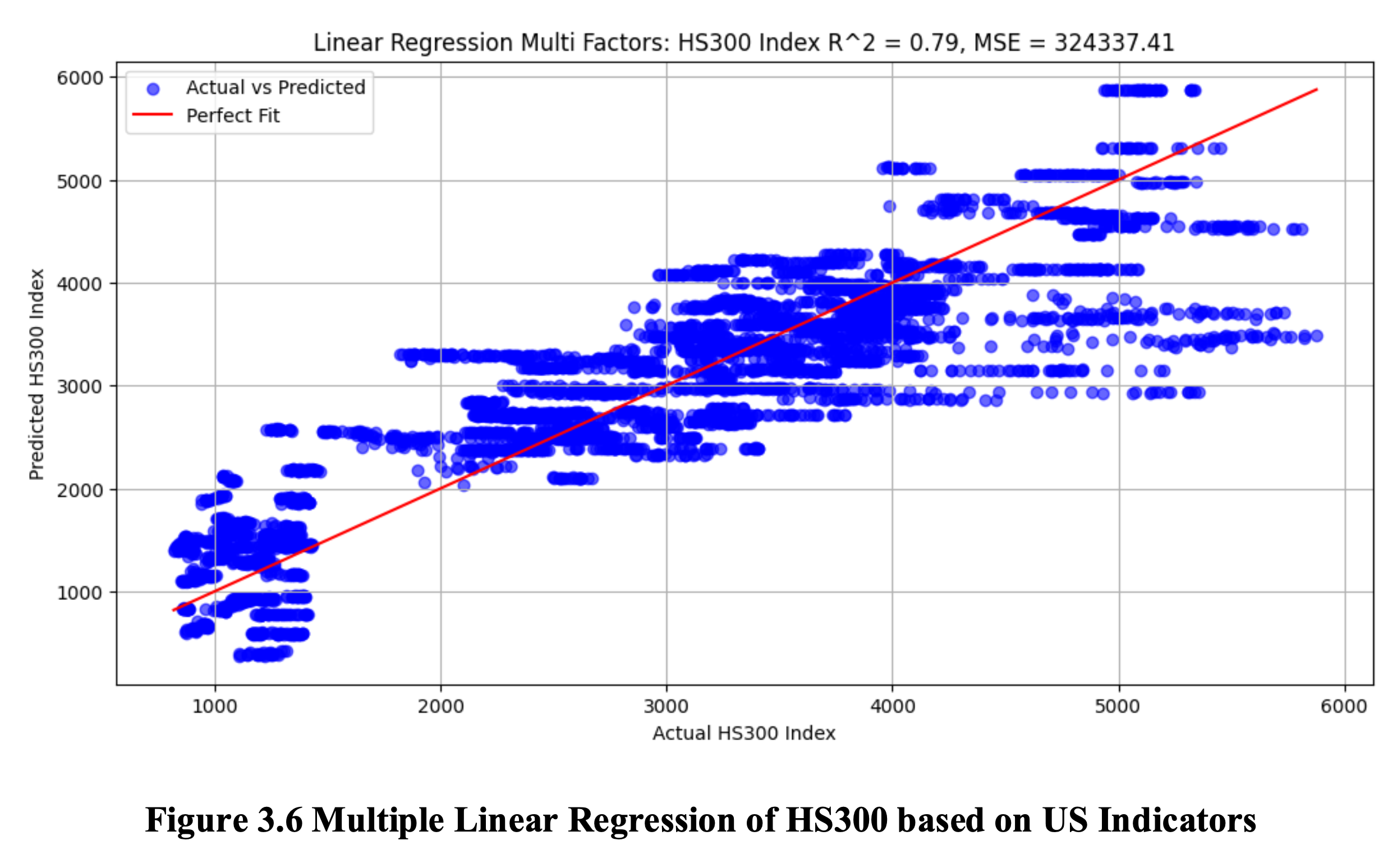
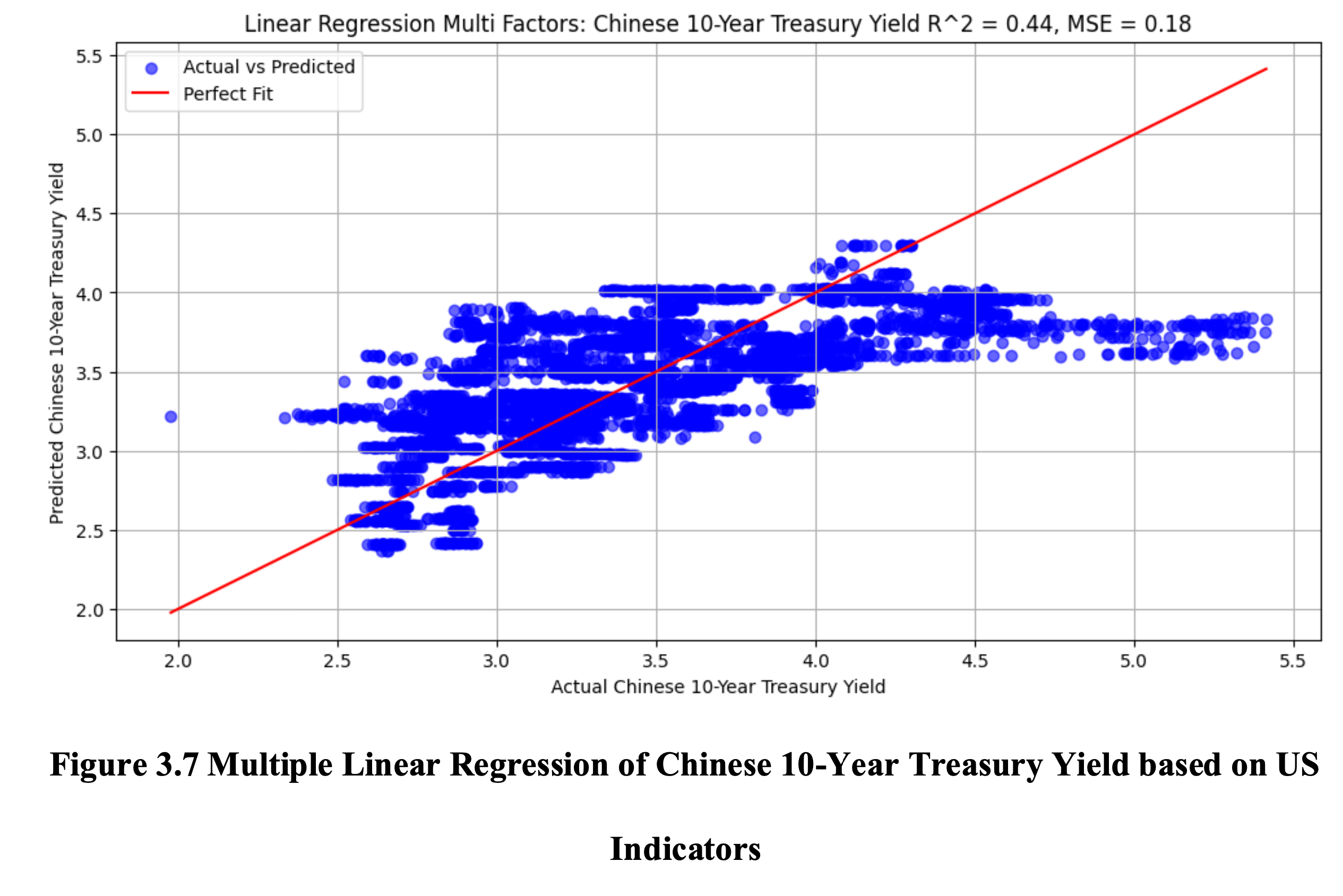
Table 3.11 presents the results of multiple linear regression of global asset prices based on US macroeconomic indicators. Most asset prices exhibit a high degree of fit with the regression model, with R-squared values exceeding 0.80. For example, the Dow Jones Index, which records the highest R-squared value of 0.9762 and all 16 macroeconomic indicators’ p-value less than 0.05 (Figure 3.5), highlights a strong correlation between the US stock market and macroeconomic conditions, reinforcing its role as a barometer of the national economy. However, HS300 Index (沪深 300) and the Chinese 10-year treasury yield, which shows a relatively low fit of 0.7872 and 0.4440 respectively (Figure 3.6, 3.7).

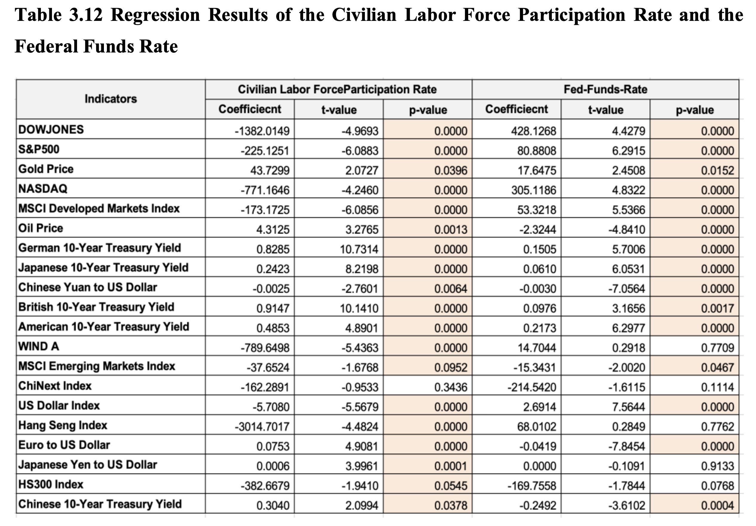
In addition, it is found that the Civilian Labor Force Participation Rate and the Federal Funds Rate are the two most significant ones among all the macroeconomic factors. As illustrated in Table 3.12, both variables exhibit significant impacts on the majority of asset prices. The Civilian Labor Force Participation Rate, defined as the percentage of individuals aged 16 and above who are either employed or actively seeking employment, is inversely correlated with most asset prices. This inverse relationship can be attributed to the wealth effect—wherein increased household wealth reduces individuals’ motivation to participate in the labor market—and to surplus labor supply, which exerts downward pressure on wages and influences market dynamics. Conversely, the Federal Funds Rate exhibits a positive correlation with asset prices. This relationship arises due to market expectations, wherein participants adjust their investment strategies in anticipation of changes in the federal funds rate, as well as global capital flows, since a higher federal funds rate enhances the attractiveness of U.S. assets to international investors by offering more competitive yields.

3.4.2 Multi-factors Regression based on China’s Macroeconomic Indicators

We hypothesize the reason of the poor regression performance of HS300 and the Chinese 10-Year Treasury Yield in the last section is attribute to Chinese assets being more heavily influenced by domestic macroeconomic indicators rather than by U.S. factors. To test this hypothesis, we introduce 7 Chinese macroeconomic indicators into our analysis.

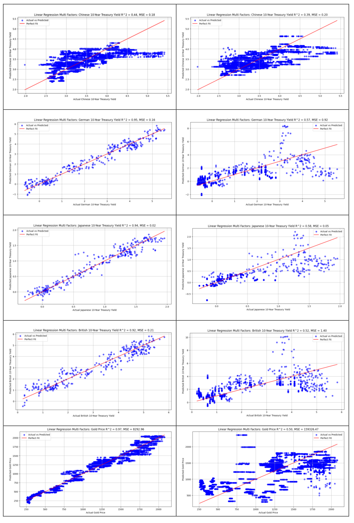
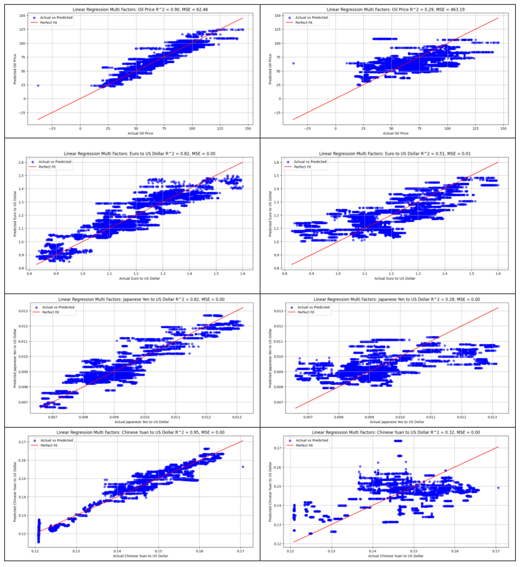
Table 3.13 presents the results of multiple linear regressions between these Chinese macroeconomic indicators and the 20 global assets prices. The findings are not satisfactory, with overall regression performance showing relatively low R² values, ranging approximately between 0.2 and 0.6. Notably, the regression results for China-related assets, such as HS300, Hang Seng Index, Chinese Yuan to US Dollar, and the Chinese 10-Year Treasury Yield, are particularly poor.

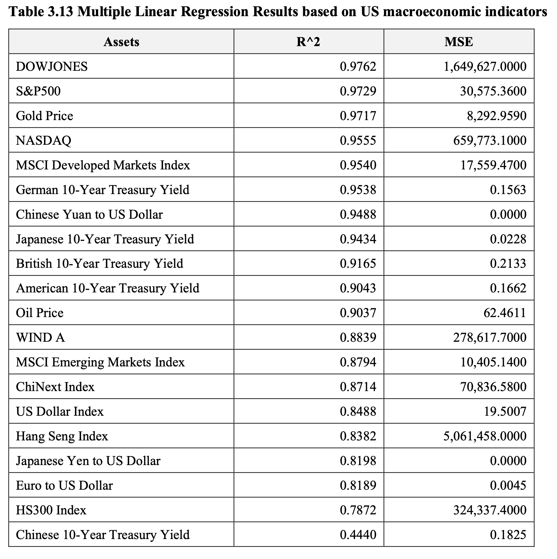
The underperformed results could be attributed to several factors. Firstly, the dynamics of Chinese assets may be influenced by non-linear relationships or structural breaks that are not well captured by linear regression models. Secondly, Chinese financial markets may be subject to unique policy interventions or regulatory factors that are not fully reflected in the selected macroeconomic indicators. Thirdly, the relatively short time series or limited variability of the data could constrain the model’s ability to detect robust relationships.

4. Conclusion

In conclusion, this report provides a comprehensive analysis of 20 global core assets, focusing on their performance, interrelationships, and macroeconomic drivers.

Firstly, the analysis recalculated asset performance during the last four Federal Reserve rate-cut cycles, correcting data inaccuracies and filling gaps from Haitong Securities’ report. Findings reveal that equities experienced sharp declines during recession-linked cycles but showed resilience during stable periods. Bonds and commodities, such as gold, displayed consistent safe-haven dynamics, while forex markets responded subtly to macroeconomic conditions.

Secondly, regression analysis, including both linear and polynomial techniques, uncovered strong correlations among closely related indices, such as the S&P 500 and Nasdaq, as well as government bond yields across developed economies. These correlations reflect both market interdependence and shared drivers.

Lastly, multi-factor regression highlighted the strong influence of U.S. macroeconomic indicators, especially the Federal Funds Rate and Civilian Labor Force Participation Rate, on global asset prices. However, Chinese financial assets exhibited poor fits with both domestic and global macroeconomic variables, emphasizing the need for localized factors and tailored modeling approaches.

In summary, this report provides valuable insights into the complexity of global asset interactions and the macroeconomic influences. Future research could adopt machine learning techniques to enhance predictive modeling and explore additional factors driving asset behavior.

Appendices

Apendix A: Data Source of Assets’ Prices

Appendix B: Data Source of Macroeconomic Indicators

Appendix C: Regression of High-correlated Pairs

Appendix D: Regression based on Macroeconomic Indicators